Worksheet 2 🐼

Tabular Data and Potential Outcomes

—TODO your name here

Collaboration Statement

• TODO brief statement on the nature of your collaboration.

• TODO your collaborator’s names here.

Learning Objectives

• Practice tabular data manipulation through pandas

• Learn more about the potential outcomes framework for causal inference

• Familiarization with mathematical operations on potential outcomes

• Familiarization with Gradescope’s autograder

Note

Before you begin Please go to Edit -> Clear Outputs of All Cells so you can run the code cells yourself!

1. pandas and tabular data [2 pts]

To familiarize ourselves with working with tabular data, we will use the pandas library and work with the National Health and Nutrition Examination Survey (NHANES) dataset. NHANES is a large, national survey that measures the health and nutrition of adults and children in the United States.

The NHANES dataset is frequently used in observational studies, where there is no intervention or manipulation of the data like a randomized experiment. We’ll cover these type of studies in a few weeks. For now, we’ll use pandas to answer some descriptive questions about the data.

pandas basics

Pandas is the defacto Python framework for working with tabular data, and it is supported by a large ecosystem of libraries, including seamless integration with numpy. Pandas provides two main data structures:

• DataFrame: a 2-dimensional data structure often used to represent a table with rows and named columns.

• Series: a 1-dimensional, labelled array, often used to represent a single column or row in a DataFrame

Pandas dataframes allow for the datatypes of the columns to be mixed. Let’s create a couple of examples by running the code cells below:

import numpy as np

# the standard import idiom for pandas
import pandas as pd

# Create a series from a list, note how there can 'nan' (missing) values
review_scores = pd.Series([4, np.nan, 2, 3])

# Note that the series can be of different data types
review_text = pd.Series(['I liked it', 'It was awful', 'Bland', 'Pretty good'])

# pandas will automatically assign a data type (dtype) to the series
review_scores

0    4.0
1    NaN
2    2.0
3    3.0
dtype: float64

Note

np.nan is a special value in pandas that represents missing data. A critical part of the data science workflow in practice is handling missing data, as results can change dramatically when missing data is not handled properly.

We can then create a dataframe by passing in a dictionary of series, where the keys are the column names:

df = pd.DataFrame({'review_scores': review_scores, 'review_text': review_text})

# Print the dataframe
df

	review_scores	review_text
0	4.0	I liked it
1	NaN	It was awful
2	2.0	Bland
3	3.0	Pretty good

Alternatively, we can create a dataframe from a dictionary of lists, which can sometimes be convenient:

# this code produces the same dataframe as before
df = pd.DataFrame({'review_scores': [4, np.nan, 2, 3], 
                   'review_text': ['I liked it', 'It was awful', 'Bland', 'Pretty good']})

For high-level inspection of the dataframe, we can use the following functions and attributes:

• df.head(): returns the first 5 rows of the dataframe

• df.tail(): returns the last 5 rows of the dataframe

• df.info(): returns a summary of the dataframe, including the number of rows, columns, and the data types of each column

• df.columns: returns the column names of the dataframe

• df.shape: returns the number of rows and columns in the dataframe

• df.dtypes: returns the data types of each column

You can play around with the dataframe in the cell below:

# the shape is a tuple of (num rows, num columns)
df.shape

(4, 2)

Often times we’ll be working with pre-existing datasets. Here, we’ll use a pre-loaded version of the NHANES dataset, which is available in the nhanes package.

Note

To load data from files manually, pandas provides various pd.read_* functions. For example, pd.read_csv loads (comma-separated values) CSV files. See pandas’ I/O documentation for more options. However, for the purposes of this worksheet, we’ll use a 3rd party package to load in NHANES because it is a complex dataset.

# load the NHANES data and metadata using pre-built functions
from nhanes.load import load_NHANES_data, load_NHANES_metadata

nhanes_df = load_NHANES_data()

nhanes_df.info()

<class 'pandas.core.frame.DataFrame'>
Index: 8366 entries, 93703.0 to 102956.0
Columns: 197 entries, GeneralHealthCondition to TimesLost10LbsOrMoreToLoseWeight
dtypes: float64(161), object(36)
memory usage: 12.6+ MB

From above, we see that the dataframe has 8,366 rows and 197 columns. Here, each row represents a survey respondent, and each column represents a survey question that was asked.

Taking a look at the columns, we see that there are a wide range of health-related questions that were asked:

# .values returns the column names as a numpy array
# nhanes_df.columns.values

Data cleaning

To select a single column, we can square bracket indexing, as if we were acessing a dictionary:

# Selects the 'GeneralHealthCondition' column and prints the first 5 rows
nhanes_df['GeneralHealthCondition'].head()

SEQN
93703.0          NaN
93704.0          NaN
93705.0         Good
93706.0    Very good
93707.0         Good
Name: GeneralHealthCondition, dtype: object

When initially exploring a dataset, it is often useful to see the unique values in a column:

# Get the unique values in the 'GeneralHealthCondition'
nhanes_df['GeneralHealthCondition'].unique()

array([nan, 'Good', 'Very good', 'Fair or', 'Excellent', 'Poor?'],
      dtype=object)

Notice two things about the GeneralHealthCondition column:

• There are some missing values in the column, represented as nan

• There are two values that seem to be typos: Poor? and Fair or

To simplify our analysis, we can remove the rows with missing values via dropna():

# remove rows with missing values in the 'GeneralHealthCondition' column, resulting in a new dataframe
nhanes_df = nhanes_df.dropna(subset=['GeneralHealthCondition'])

We can also correct the typos using replace():

# replace the typos with the correct values
nhanes_df['GeneralHealthCondition'] = nhanes_df['GeneralHealthCondition'].replace({'Poor?': 'Poor', 'Fair or': 'Fair'})

# print the unique values again to see the changes
nhanes_df['GeneralHealthCondition'].unique()

array(['Good', 'Very good', 'Fair', 'Excellent', 'Poor'], dtype=object)

Tip

Notice how in both operations, we reassign the result back to nhanes_df or a column in nhanes_df, which is a common pattern in pandas – operations often return a new dataframe or column, and we need to reassign the result back to the original variable if we want to keep the changes.

Indexing and assignment

The square bracket indexing can be generalized to selecting multiple columns:

# Selects multiple columns and prints the first 10 rows
cols = ['GeneralHealthCondition', 'AgeInYearsAtScreening', 'SmokedAtLeast100CigarettesInLife', 'WeightKg', 'VigorousRecreationalActivities']
nhanes_df[cols].head(10)

	GeneralHealthCondition	AgeInYearsAtScreening	SmokedAtLeast100CigarettesInLife	WeightKg	VigorousRecreationalActivities
SEQN
93705.0	Good	66.0	1.0	79.5	0.0
93706.0	Very good	18.0	0.0	66.3	0.0
93707.0	Good	13.0	NaN	45.4	NaN
93708.0	Good	66.0	0.0	53.5	0.0
93711.0	Very good	56.0	0.0	62.1	1.0
93712.0	Good	18.0	1.0	58.9	1.0
93713.0	Very good	67.0	1.0	74.9	0.0
93714.0	Good	54.0	1.0	87.1	0.0
93715.0	Fair	71.0	1.0	65.6	1.0
93716.0	Very good	61.0	1.0	77.7	1.0

Just like numpy, we can also use boolean indexing to select portions of the dataframe based on a condition:

# Selects respondents who have smoked at least 100 cigarettes in their life
sel_df = nhanes_df[nhanes_df['SmokedAtLeast100CigarettesInLife'] == 1]

sel_df[cols].head(10)

	GeneralHealthCondition	AgeInYearsAtScreening	SmokedAtLeast100CigarettesInLife	WeightKg	VigorousRecreationalActivities
SEQN
93705.0	Good	66.0	1.0	79.5	0.0
93712.0	Good	18.0	1.0	58.9	1.0
93713.0	Very good	67.0	1.0	74.9	0.0
93714.0	Good	54.0	1.0	87.1	0.0
93715.0	Fair	71.0	1.0	65.6	1.0
93716.0	Very good	61.0	1.0	77.7	1.0
93717.0	Very good	22.0	1.0	74.4	0.0
93726.0	Very good	67.0	1.0	74.3	0.0
93727.0	Excellent	70.0	1.0	62.7	0.0
93729.0	Fair	42.0	1.0	82.8	0.0

We can then use the value_counts function to get the frequency of each category in a column:

print(sel_df['GeneralHealthCondition'].value_counts())

# normalize=True to get the proportion of each category
# dropna=False to include missing values as part of counts
print(sel_df['GeneralHealthCondition'].value_counts(dropna=False, normalize=True))

GeneralHealthCondition
Good         899
Fair         544
Very good    430
Excellent    126
Poor         103
Name: count, dtype: int64
GeneralHealthCondition
Good         0.427688
Fair         0.258801
Very good    0.204567
Excellent    0.059943
Poor         0.049001
Name: proportion, dtype: float64

Tip

Many pandas operations by default drop na values, so be careful to double check what the default behavior is!

1.1. How would we get the general health condition proportions of respondents who have engaged in vigorous recreational activities (1 = yes, 0 = no)? Write code to do this below:

# TODO your code here

What proportion of respondents who have engaged in vigorous recreational activities report being in excellent health?

Your response: TODO

These boolean conditions can be combined using the & (AND), | (OR), and ~ (NOT) operators. Additionally, there are some special functions that can be used to select data based on a condition:

# Combining conditions: respondents who are 18 or older and have engaged in vigorous recreational activities
nhanes_df[(nhanes_df['AgeInYearsAtScreening'] >= 18) & (nhanes_df['VigorousRecreationalActivities'] == 1)] 

# isin(): select rows where a column is in a list of values
nhanes_df[nhanes_df['GeneralHealthCondition'].isin(['Poor?', 'Fair or'])]

# isna(): select rows where a column is missing
nhanes_df[nhanes_df['SmokedAtLeast100CigarettesInLife'].isna()];

Tip

To avoid errors, always use parentheses when combining conditions:

• Incorrect: df[column1 == value1 & column2 == value2]

• Correct: df[(column1 == value1) & (column2 == value2)]

We can also create new columns or modify existing columns via = assignment (like we did with replace()):

# Assign a constant value to a new column where every row has the same value
nhanes_df['country'] = 'United States'

# Create a new column based on a condition of other columns
nhanes_df['is_adult'] = nhanes_df['AgeInYearsAtScreening'] >= 18

# Create a new column based on a function of other columns: calculate BMI
nhanes_df['bmi'] = nhanes_df['WeightKg'] / (nhanes_df['StandingHeightCm'] / 100) ** 2

# Print the updated dataframe
nhanes_df[['country', 'is_adult', 'AgeInYearsAtScreening', 'bmi']].head()

	country	is_adult	AgeInYearsAtScreening	bmi
SEQN
93705.0	United States	True	66.0	31.725268
93706.0	United States	True	18.0	21.476821
93707.0	United States	False	13.0	18.094455
93708.0	United States	True	66.0	23.714497
93711.0	United States	True	56.0	21.337009

1.2. Let’s practice combining these operations. Select respondents who:

• are adults AND

• report being in Excellent or Very good health AND

• are NOT missing any values in the bmi column

Write code to do this below:

# TODO your code here

How many respondents are in the selected group? How many of them have smoked at least 100 cigarettes in their life?

Your response: TODO

the .loc operator

In addition to square bracket indexing, pandas provides a powerful indexing method via the .loc operator, which allows us to select rows and columns by their labels or even boolean conditions.

Generally, the .loc operator is used to select rows and columns by their labels:

df.loc[row_label, column_label]

The loc operator borrows from the slice notation of python lists, where we can use : to select all rows or column:

# selects all rows and the 'bmi' column, returned as a series
nhanes_df.loc[:, 'bmi'].head()

SEQN
93705.0    31.725268
93706.0    21.476821
93707.0    18.094455
93708.0    23.714497
93711.0    21.337009
Name: bmi, dtype: float64

# selects all rows and the ['country', 'is_adult', 'bmi'] columns
# Note that the columns are wrapped in a list!
nhanes_df.loc[:, ['country', 'is_adult', 'bmi']].head()

	country	is_adult	bmi
SEQN
93705.0	United States	True	31.725268
93706.0	United States	True	21.476821
93707.0	United States	False	18.094455
93708.0	United States	True	23.714497
93711.0	United States	True	21.337009

Where the .loc operator becomes useful is when we want to compactly select rows and columns based on a condition:

# selects rows where the 'bmi' column is greater than 25, and returns the 'bmi' and 'is_adult' columns
nhanes_df.loc[nhanes_df['bmi'] > 25, ['bmi', 'is_adult']].head()

	bmi	is_adult
SEQN
93705.0	31.725268	True
93714.0	39.872116	True
93716.0	30.657370	True
93719.0	26.009064	False
93721.0	35.882948	True

This selection can be used to modify columns based on a condition:

# set the 'bmi' column to np.nan for all rows where the 'is_adult' column is False
nhanes_df.loc[nhanes_df['is_adult'] == False, 'bmi'] = np.nan

# print the updated dataframe
nhanes_df[['bmi', 'is_adult']].head()

	bmi	is_adult
SEQN
93705.0	31.725268	True
93706.0	21.476821	True
93707.0	NaN	False
93708.0	23.714497	True
93711.0	21.337009	True

1.3. Common age cutoffs that are used in health policy studies are 18 and 65 – 18 is when people are legally considered adults in the United States, and 65 is when they are eligible for Medicare health insurance. Create a new column age_category using the AgeInYearsAtScreening column and the .loc operator that makes the following assignments:

• 'child': age < 18

• 'adult': 18 <= age < 65

• 'senior': age >= 65

# TODO your code here

How many respondents are in the ‘senior’ age category?

Your response: TODO

Grouping and transformation

The groupby() function is a powerful tool for performing aggregations on subsets of the dataframe. We pass in one or more columns as the by argument, which then divides the original Dataframe based on the unique values of the column(s). We then often apply an aggregation function to each group, resulting in a new dataframe.

We can replicate value_counts() with groupby() and the size() aggregation function:

# Count number of people in each health condition category
print(nhanes_df.groupby(by='GeneralHealthCondition').size())

GeneralHealthCondition
Excellent     619
Fair         1175
Good         2454
Poor          172
Very good    1544
dtype: int64

We can also compute summary statistics like mean(), std(), median(), min(), max() on each group:

# Calculate mean BMI by general health condition
nhanes_df.groupby(by='GeneralHealthCondition')['bmi'].mean()

GeneralHealthCondition
Excellent    26.518102
Fair         31.889146
Good         30.176114
Poor         34.366233
Very good    27.744468
Name: bmi, dtype: float64

We can also group by multiple columns, which then groups the dataframe by the unique cross-product of the columns:

# Calculate mean BMI by general health condition and vigorous recreational activities
# as_index=False keeps the groupby columns as columns in the resulting dataframe
nhanes_df.groupby(by=['GeneralHealthCondition', 'VigorousRecreationalActivities'], as_index=False)['bmi'].mean()

	GeneralHealthCondition	VigorousRecreationalActivities	bmi
0	Excellent	0.0	27.303422
1	Excellent	1.0	25.496384
2	Fair	0.0	31.804008
3	Fair	1.0	32.433563
4	Good	0.0	30.266370
5	Good	1.0	29.861264
6	Poor	0.0	34.507856
7	Poor	1.0	31.169604
8	Very good	0.0	28.349808
9	Very good	1.0	26.684116

To apply multiple aggregation functions, we can pass in a dictionary of columns as keys and functions as values to agg():

# Calculate mean, min, max for BMI and median household income by general health condition
nhanes_df.groupby(by='GeneralHealthCondition').agg({'bmi': ['mean', 'min', 'max'], 'AnnualHouseholdIncome': 'median'})

	bmi			AnnualHouseholdIncome
	mean	min	max	median
GeneralHealthCondition
Excellent	26.518102	16.111752	57.266546	60000.0
Fair	31.889146	15.469697	72.555993	30000.0
Good	30.176114	15.455268	86.160237	50000.0
Poor	34.366233	14.910611	84.404111	30000.0
Very good	27.744468	14.818824	57.689838	60000.0

1.4. Generate a table that groups by:

• GeneralHealthCondition

• SmokedAtLeast100CigarettesInLife

and calculates the mean of the following columns:

• EverToldYouHavePrediabetes: 0 = no, 1 = yes

• EverToldYouHadHeartAttack: 0 = no, 1 = yes

Note

The mean of a binary column is equivalent to the proportion of 1s in the column.

# TODO your code here

Which subgroup of health conditions and smoking status has the highest proportion of people who have been told they have had a heart attack?

Your response: TODO

Note

For more on pandas operations, see this quickstart guide and the associated links within it.

2. Reading: Neal 2020 [1 pt]

Read the following sections of Neal 2020: An Introduction to Causal Inference and answer the questions below:

• Sections 2.1 - 2.3.2

• Section 2.3.5

Reading Notes

• Don’t worry too much about the causal graphs shown in the margin, as we’ll cover causal graph formalisms in upcoming classes.

• The notation \(\triangleq\) is used to denote “is defined as”. For example, Equation 2.1 \(\tau_i \triangleq Y_i(1) - Y_i(0)\) means that the individual treatment effect for unit \(i\) is defined as \(Y_i(1) - Y_i(0)\).

• A mathematical identity we’ll need for the derivations is linearity of expectation. This states that for any random variables \(X\) and \(Y\) and constant \(a\):

\[ E[X + Y] = E[X] + E[Y] \]

\[ E[aX] = aE[X] \]

• Implications of two variables \(X\) and \(Y\) being independent (written \(X \perp Y\)) are that:

\[ E[X | Y=y] = E[X] \]

\[ E[XY] = E[X]E[Y] \]

• The consistency assumption (Assumption 2.5) allows us to define the observed outcome \(Y\) with binary treatment \(T\) as follows:

\[ Y = T \cdot Y(1) + (1-T) \cdot Y(0) \]

2.1. State the fundamental problem of causal inference in your own words.

Your Response: TODO

2.2. These sections of Neal 2020 cover three key assumptions that allow us to identify (definition 2.1, p. 10) the average treatment effect (ATE) of a binary treatment:

• ignorability / exchangeability (Assumption 2.1, p. 9)

• no interference (Assumption 2.4, p. 13)

• consistency (Assumption 2.5, p. 14)

Below is a restatement of the ATE derivation. State which mathematical identities and assumptions are used on each line:

\[\begin{split} ATE &= E[Y(1) - Y(0)]\\ &= E[Y(1)] − E[Y(0)], \text{ from TODO} \\ &= E[Y(1) | T = 1] − E[Y(0) | T = 0], \text{ from TODO} \\ &= E[Y | T = 1] − E[Y | T = 0] \text{ from TODO} \end{split}\]

2.3. The no interference assumption states that the potential outcomes for one unit are unaffected by the treatment assignment of other units. Breaking down Neal’s example on p. 13, suppose that you are unit 1 and your friend is unit 2. If your friend gets a dog (\(t_2 = 1\)), we can then examine your potential outcomes:

\[\begin{split} &Y_1(t_1, t_2), \text{ potential outcomes for unit 1} \\ &Y_1(0, 1), \text{ you don't get a dog, but your friend does} \\ &Y_1(1, 1), \text{ you and your friend get a dog} \end{split}\]

The argument is that it is likely that the potential outcomes for your happiness are affected by your friend’s choice to get a dog: perhaps you’ll already be happier if your friend gets a dog because you get to play with them, or perhaps you’re allergic to dogs so you have to see your friend less often, etc. This leads to a violation of the no interference assumption where your potential outcomes are no longer just a function of your own treatment assignment \(t_1\):

\[\begin{split} Y_1(0, 1) \neq Y_1(0) \\ Y_1(1, 1) \neq Y_1(1) \end{split}\]

Neal then states that “violations of the no interference assumption are rampant in network data,” e.g. friend groups like the dog example above, social networks, or transportation networks (think roads, subway lines, airports). Give an example of a setting along with a treatment \(T\) and outcome \(Y\) where you think the no interference assumption is likely to be violated.

Your Response:

• Treatment: TODO

• Outcome: TODO

• Reasoning: TODO

3. Causal inference as a missing data problem [1 pt]

Let’s now put the conceptual ideas around potential outcomes together with our table manipulation practice in pandas.

Our framework for causal inference is that there is there is a causal “ground truth” table of potential outcomes for each unit. With our example from class, we might be interested in studying the effect of taking aspirin \(T\) (\(T=1\) means taking aspirin, \(T=0\) means not taking aspirin) on headaches \(Y\) (\(Y=1\) means having a headache, \(Y=0\) means not having a headache). The potential outcomes then correspond to:

\[\begin{split} Y(0) = \text{what the outcome } \textit{would have been} \text{ if } T = 0 \\ Y(1) = \text{what the outcome } \textit{would have been} \text{ if } T = 1 \end{split}\]

We then have a table of potential outcomes for each unit, where each row is a unit and each column is a potential outcome:

\[\begin{split} \begin{array}{c|c|c|c} \text{Unit } i & T & Y(0) & Y(1) \\ \hline 1 & 0 & 1 & 1 \\ 2 & 1 & 1 & 0 \\ 3 & 0 & 1 & 0 \\ 4 & 1 & 0 & 0 \\ \end{array} \end{split}\]

The problem is that we are not omniscient, nor do we have a time machine, so we only observe one realized outcome \(Y\) for each unit. There are thus missing values in the table of the data we actually observe:

\[\begin{split} \begin{array}{c|c|c|c|c} \text{Unit } i & T & Y(0) & Y(1) & Y \\ \hline 1 & 0 & 1 & \text{nan} & 1 \\ 2 & 1 & \text{nan} & 0 & 0 \\ 3 & 0 & 1 & \text{nan} & 1 \\ 4 & 1 & \text{nan} & 0 & 0 \\ \end{array} \end{split}\]

The challenge in causal inference is to try to construct causal estimates when we only have the observed data. Throughout this course we’ll use our ability to simulate different data generating processes in code to understand the properties of causal inference methods, and when they can or cannot identify the causal effect.

We’ll start by writing a utility function that takes treatment assignments and a ground truth table of potential outcomes, and generates the realized outcomes.

Hint

To construct the observed outcome \(Y\), look to how we defined \(Y\) under the consistency assumption.

def generate_observed_df(po_df, treatments):
    """
    Generates a dataframe of realized outcomes from a ground truth table of potential outcomes and treatment assignments.
    The unobserved potential outcomes are set to np.nan.
    
    Args:
        po_df (pd.DataFrame): a dataframe of potential outcomes with columns 'Y0' and 'Y1'
        treatments (pd.Series): a series of treatment assignments with the same length as po_df

    Returns:
        pd.DataFrame: a dataframe of realized outcomes with columns 'T', 'Y0', 'Y1', and 'Y'
    """
    assert po_df.shape[0] == treatments.shape[0], "The number of rows in po_df and treatments must match"
    
    # TODO your code here
    observed_df = po_df.copy()

    return observed_df

# Generate some simple test data, matching the example above
treatments = pd.Series([0, 1, 0, 1])
po_df = pd.DataFrame({'Y0': [1, 1, 1, 0], 'Y1': [1, 0, 0, 0]})
observed_df = generate_observed_df(po_df, treatments)
assert 'Y' in observed_df.columns, "The observed dataframe does not have a 'Y' column"

---------------------------------------------------------------------------
AssertionError                            Traceback (most recent call last)
Cell In[29], line 24
     22 po_df = pd.DataFrame({'Y0': [1, 1, 1, 0], 'Y1': [1, 0, 0, 0]})
     23 observed_df = generate_observed_df(po_df, treatments)
---> 24 assert 'Y' in observed_df.columns, "The observed dataframe does not have a 'Y' column"

AssertionError: The observed dataframe does not have a 'Y' column

Tip

This is the first auto-graded function in the course – there will be no submission limit so feel free to try multiple times. We will frequently provide some simple test cases via assert statements to check your function. The syntax for assert statements is as follows:

assert bool_expression, description

where the bool_expression is a boolean expression that tests some condition, and the description is a string that will be displayed if the assertion fails (evaluates to False).

You are encouraged to write your own test cases as well for your functions!

Takeaway

This transformation from the ground truth table of potential outcomes to the observed data is a key step in thinking about causal quantities. If only we had the ground truth table, we could directly estimate quantities like \(E[Y(1)]\) and \(E[Y(0)]\). However, since we only have the observed data, we need to make assumptions, like the ones covered in the Neal reading, in order to “reconstruct” those quantities. This is the process of identifying the causal effect. See the figure below:

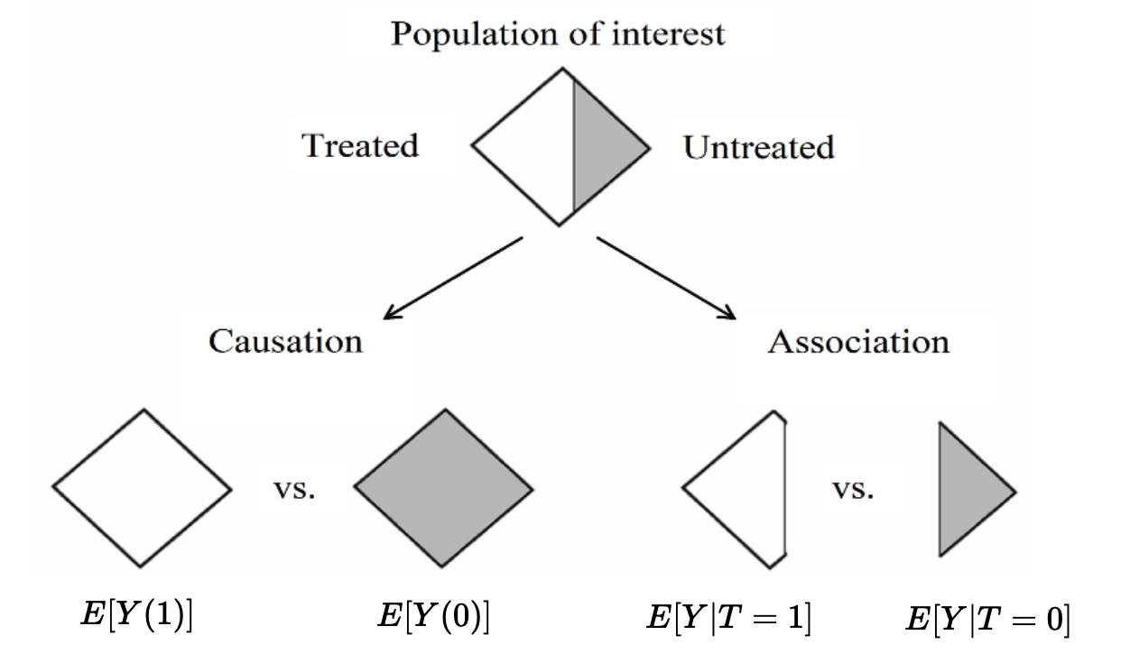
Fig. 1 Adapted from Hernán and Robins 2020 1.1

We saw from the Neal reading that the assumptions made in a randomized experiment allow for us to identify the causal effect, i.e. reconstruct \(E[Y(1)]\) from \(E[Y|T=1]\), and \(E[Y(0)]\) from \(E[Y|T=0]\). You may sometimes hear that “association is causation, in a randomized experiment.”

The crux of the “design” step in the causal roadmap generally involves evaluating what assumptions we need in order to perform identification, and whether those assumptions are reasonable to make.

4. Reflection [1 pt]

4.1 How much time did it take you to complete this worksheet? How long did it take you to read the selected sections of Neal 2020?

Your Response: TODO

4.2 What is one thing you have a better understanding of after completing this worksheet and going though the class content this week? This could be about the concepts, the reading, or the code.

Your Response: TODO

4.3 What questions or points of confusion do you have about the material covered in the past week of class?

Your Response: TODO

Tip

Don’t forget to check that all of the TODOs are filled in before you submit!

Acknowledgements

Portions of this worksheet are adapted from Bhargavi’s study notes on pandas. This worksheet also uses Russ Poldrack’s nhanes package, which processes the NHANES dataset into a convenient pandas dataframe.