Activity 16 Solution: Causal Trees#
2025-04-24
import pandas as pd
import numpy as np
import matplotlib.pyplot as plt
from econml.dml import CausalForestDML
from econml.cate_interpreter import SingleTreeCateInterpreter
Run the cell below to load in the data. We have the following variables:
age: age of the customerincome: income of the customer, in $100khas_membership: whether the customer has a membership to the online music platformavg_hours: average number of hours per week the customer has spent on the platformdemand: outcome variable – sales of songs on the platformT: treatment (1 if the customer was given a discount, 0 otherwise)
customer_data = pd.read_csv('~/COMSC-341CD/data/customer_data.csv')
customer_data.head()
| age | income | has_membership | avg_hours | T | demand | |
|---|---|---|---|---|---|---|
| 0 | 53 | 0.960863 | 1 | 1.834234 | 0 | 3.917117 |
| 1 | 54 | 0.732487 | 0 | 7.171411 | 0 | 11.585706 |
| 2 | 33 | 1.130937 | 0 | 5.351920 | 0 | 24.675960 |
| 3 | 34 | 0.929197 | 0 | 6.723551 | 0 | 6.361776 |
| 4 | 30 | 0.533527 | 1 | 2.448247 | 1 | 12.624123 |
A more robust variant of causal tree prediction is to fit multiple trees and take the average of the predictions. This is known as the causal forest, and it just like a random forest model in machine learning. This is implemented in EconML as the CausalForestDML class. Initialize the model as follows:
causal_forest = CausalForestDML(criterion='mse', # use mean squared error as the loss function
                                honest=True, # use honest sample splitting
                                discrete_treatment=True # treatment is binary
                                )
Then call causal_forest.fit() with the following arguments:
X: the features given bycustomer_data[covariates]T: the treatment column given bycustomer_data['T']Y: the outcome column given bycustomer_data['demand']
The model may take ~1-2 minutes to fit.
covariates = ['age', 'income', 'has_membership', 'avg_hours']

# TODO initialize causal forest model
causal_forest = CausalForestDML(criterion='mse', # use mean squared error as the loss function
                                honest=True, # use honest sample splitting
                                discrete_treatment=True # treatment is binary
                                )

# TODO fit the model with the appropriate parameters
causal_forest.fit(X=customer_data[covariates],
                  T=customer_data['T'],
                  Y=customer_data['demand'])
<econml.dml.causal_forest.CausalForestDML at 0x349f5b950>
You can then check the average treatment effect (ATE) via the causal_forest.ate_ attribute.
print("ATE: ", causal_forest.ate_)
ATE: [1.60537994]
Takeaway (click once you’ve completed the code)
The ATE estimate you should get is around 1.35, which can be interpreted as: on average, giving a discount to a customer increases the number of songs purchased by 1.35.
Next, we’ll summarize the causal forest model into a single causal tree using the SingleTreeCateInterpreter class. Initialize the interpreter with the parameter max_depth=2.
Then, call the interpret() method with the following arguments:
cate_estimator: our fitted causal forest modelX: the features given bycustomer_data[covariates]
# TODO initialize the causal tree interpreter
cate_tree = SingleTreeCateInterpreter(max_depth=2)

# TODO fit the interpreter with the causal forest model
cate_tree.interpret(causal_forest, X=customer_data[covariates])
<econml.cate_interpreter._interpreters.SingleTreeCateInterpreter at 0x34adb1ad0>
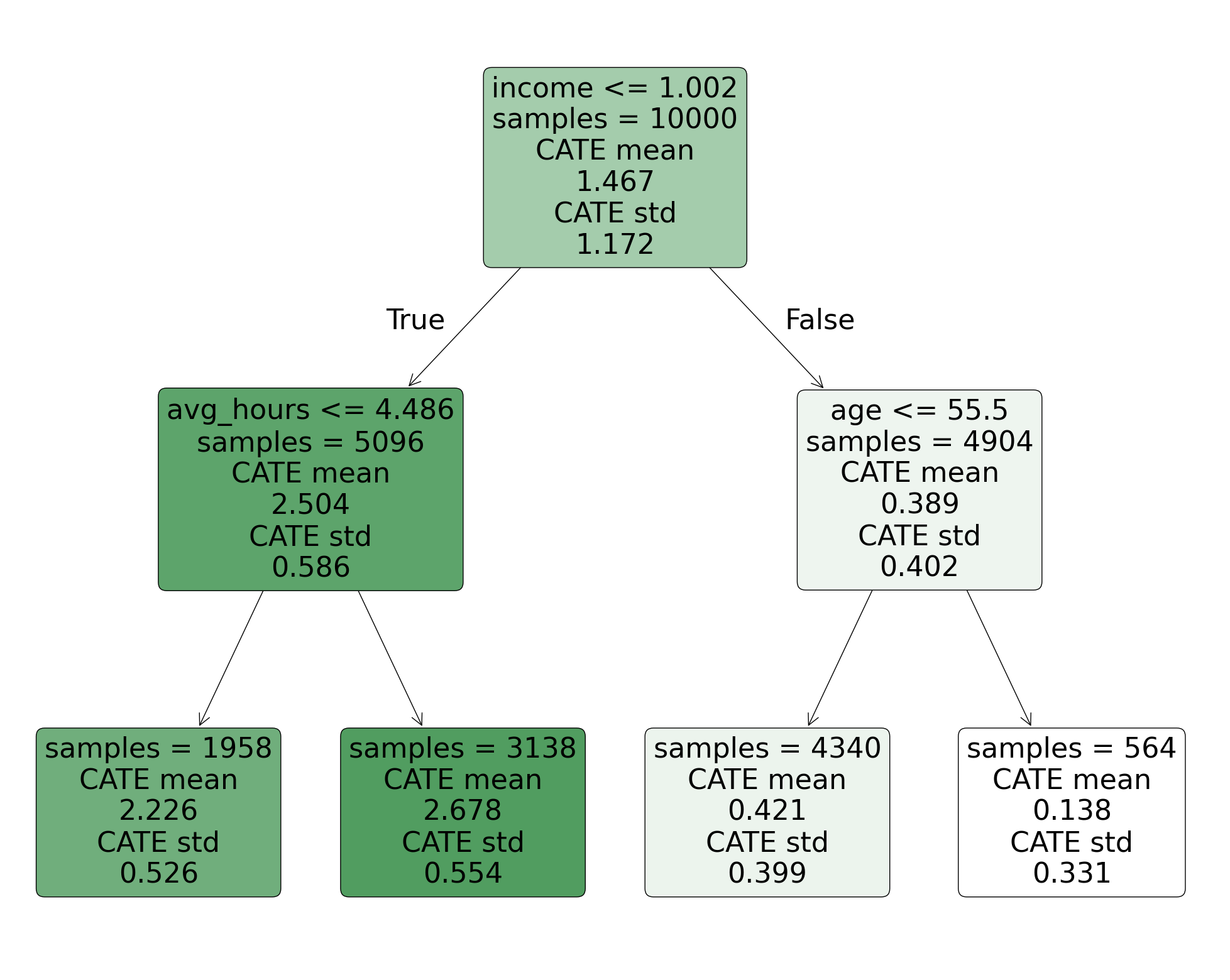
Finally, uncomment and run the cell below to plot the causal tree. According to the tree, which subgroup of customers buys the most product after being given a discount?
Your response: pollev.com/tliu
# resizes the plot to fit the causal tree
plt.figure(figsize=(25, 20))
cate_tree.plot(feature_names=covariates)
Acknowledgements#
This activity uses tutorial code and data provided by the EconML package.