Activity 17: Panel data Solutions#
import seaborn as sns
import pandas as pd
import numpy as np
import matplotlib.pyplot as plt
import statsmodels.formula.api as smf
Part 1#
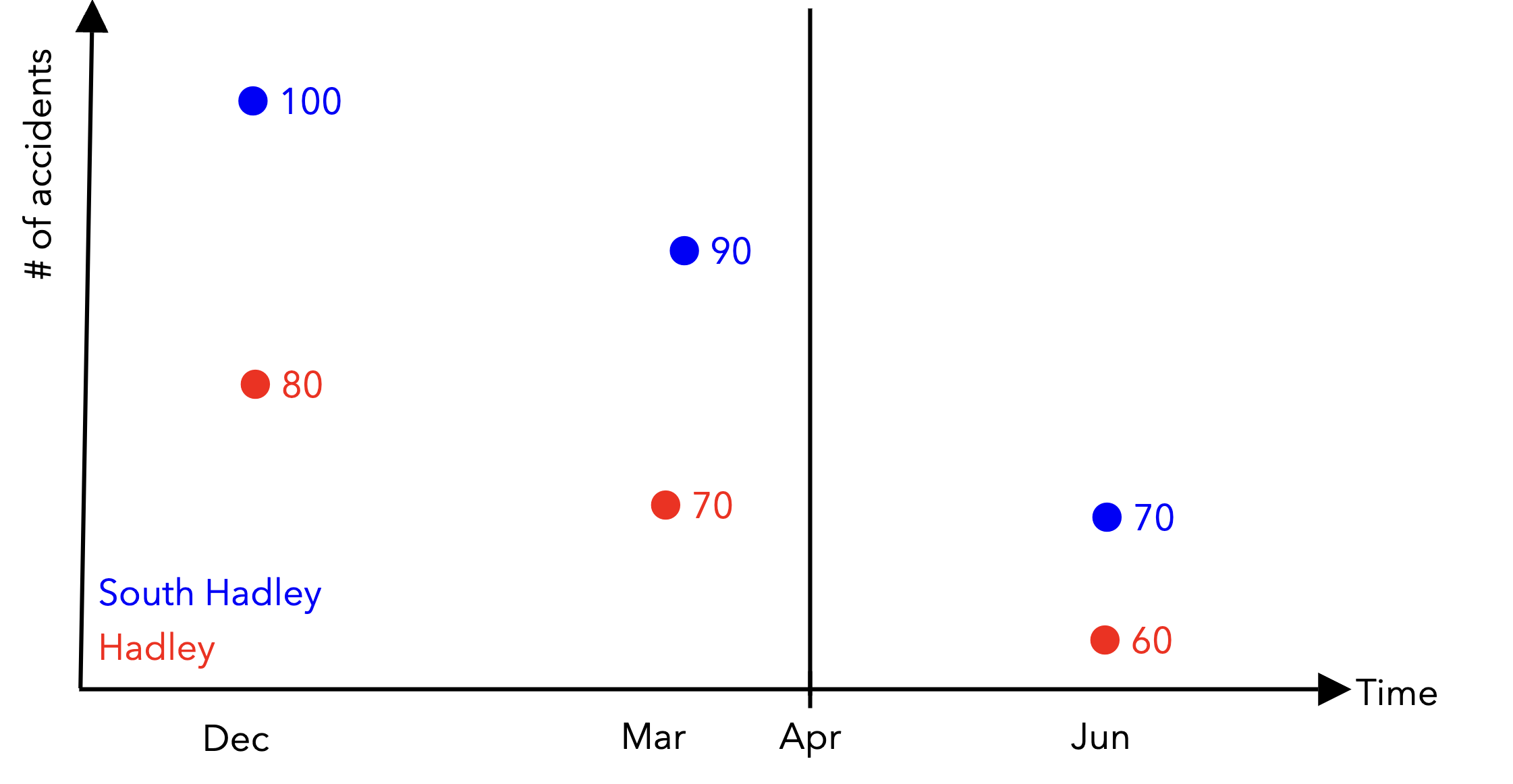
With panel data, instead of having a single row per unit in our dataframes, we have potentially multiple datapoints per unit across time. Given that:
December: \(t=1\)
March: \(t=2\)
June: \(t=3\)
We have 3 datapoints for each town. The “Post-treatment period?” column is a binary variable that is 1 if the datapoint is in the post-treatment period and 0 otherwise.
Finish populating the markdown table below with the correct values:
Unit |
Time |
Outcome |
Post-treatment period? |
|---|---|---|---|
South Hadley |
1 |
100 |
0 |
South Hadley |
2 |
90 |
0 |
South Hadley |
3 |
70 |
1 |
Hadley |
1 |
80 |
0 |
Hadley |
2 |
70 |
0 |
Hadley |
3 |
60 |
1 |
We can use pandas MultiIndex to represent the multiple indices needed for panel data. The pd.set_index() can take a list of columns to use as the new index.
traffic_df = pd.DataFrame(
    {
        'town': ['South Hadley', 'South Hadley', 'South Hadley', 'Hadley', 'Hadley', 'Hadley'],
        'time': [1, 2, 3, 1, 2, 3],
        'outcome': [100, 90, 70, 80, 70, 60],
        "post_treatment": [0, 0, 1, 0, 0, 1]
    }
)

# TODO set the index to be the['town', 'time'] columns
traffic_df = traffic_df.set_index(["town", "time"])

display(traffic_df)

# note that time and town are no longer columns
display(traffic_df.columns)
| outcome | post_treatment | ||
|---|---|---|---|
| town | time | ||
| South Hadley | 1 | 100 | 0 |
| 2 | 90 | 0 | |
| 3 | 70 | 1 | |
| Hadley | 1 | 80 | 0 |
| 2 | 70 | 0 | |
| 3 | 60 | 1 |
Index(['outcome', 'post_treatment'], dtype='object')
The multi-index is now, where the first level (level=0) is the town and the second level (level=1) is the time.
With a multi-index, the .loc method can take a tuple that specifies an index to retrieve:
# selects all the South Hadley datapoints
display(traffic_df.loc["South Hadley"])
| outcome | post_treatment | |
|---|---|---|
| time | ||
| 1 | 100 | 0 |
| 2 | 90 | 0 |
| 3 | 70 | 1 |
# selects the row for South Hadley at time 1
display(traffic_df.loc[("South Hadley", 1)])
#display(traffic_df.loc[("South Hadley", 1)])

# equivalently, we can chain the `.loc` method to filter different levels of the multi-index
display(traffic_df.loc["South Hadley"].loc[1])
#display(traffic_df.loc["South Hadley"].loc[1])
outcome           100
post_treatment      0
Name: (South Hadley, 1), dtype: int64
outcome           100
post_treatment      0
Name: 1, dtype: int64
To select rows based on the second level of the multi-index, we can use pd.xs, which takes a cross-section of the DataFrame:
# Select all rows where the second level of the multi-index (time) equals 1
traffic_df.xs(1, level=1)
| outcome | post_treatment | |
|---|---|---|
| town | ||
| South Hadley | 100 | 0 |
| Hadley | 80 | 0 |
Write a line of code to select the Hadley datapoint at time 3, and submit your answer to pollEverywhere:
display(traffic_df.loc[("Hadley", 3)])
outcome           60
post_treatment     1
Name: (Hadley, 3), dtype: int64
Part 2#
Run the cell below to load the organ donation data. The dataframe has the following columns:
State: the state name
Quarter: the quarter of data
Quarter_Num: the quarter number
Rate: the organ donation registration rate
organ_df = pd.read_csv("~/COMSC-341CD/data/organ_donations.csv")
organ_df.head(10)
| State | Quarter | Rate | Quarter_Num | |
|---|---|---|---|---|
| 0 | Alaska | Q42010 | 0.7500 | 1 |
| 1 | Alaska | Q12011 | 0.7700 | 2 |
| 2 | Alaska | Q22011 | 0.7700 | 3 |
| 3 | Alaska | Q32011 | 0.7800 | 4 |
| 4 | Alaska | Q42011 | 0.7800 | 5 |
| 5 | Alaska | Q12012 | 0.7900 | 6 |
| 6 | Arizona | Q42010 | 0.2634 | 1 |
| 7 | Arizona | Q12011 | 0.2092 | 2 |
| 8 | Arizona | Q22011 | 0.2261 | 3 |
| 9 | Arizona | Q32011 | 0.2503 | 4 |
Since the data is quarterly and begins in 2010 Q4, the first post-treatment period (after July 2011) is 2011 Q3, which corresponds to Quarter_Num = 4. Create the following columns to prepare the data for a difference-in-differences analysis:
is_california: a binary variable indicating whether the state is Californiapost_treatment: a binary variable indicating whether the quarter is after 2011 Q3 (Quarter_Num >= 4)is_treated: a binary variable indicating whether the state is California AND the quarter is after 2011 Q3
#organ_df[['State', 'is_california']].head(20)
# TODO: Create the columns
organ_df['is_california'] = organ_df.loc[:, 'State'] == 'California'
organ_df['post_treatment'] = organ_df['Quarter_Num'] >= 4
organ_df['is_treated'] = organ_df['is_california'] & organ_df['post_treatment']
organ_df[['Quarter_Num', 'post_treatment', 'State', 'is_treated']].head(20)
| Quarter_Num | post_treatment | State | is_treated | |
|---|---|---|---|---|
| 0 | 1 | False | Alaska | False |
| 1 | 2 | False | Alaska | False |
| 2 | 3 | False | Alaska | False |
| 3 | 4 | True | Alaska | False |
| 4 | 5 | True | Alaska | False |
| 5 | 6 | True | Alaska | False |
| 6 | 1 | False | Arizona | False |
| 7 | 2 | False | Arizona | False |
| 8 | 3 | False | Arizona | False |
| 9 | 4 | True | Arizona | False |
| 10 | 5 | True | Arizona | False |
| 11 | 6 | True | Arizona | False |
| 12 | 1 | False | California | False |
| 13 | 2 | False | California | False |
| 14 | 3 | False | California | False |
| 15 | 4 | True | California | True |
| 16 | 5 | True | California | True |
| 17 | 6 | True | California | True |
| 18 | 1 | False | Colorado | False |
| 19 | 2 | False | Colorado | False |
Like we did in part 1, set the index to be the ['State', 'Quarter_Num'] columns.
# TODO set the multi-index
#organ_df.set_index(TODO)
Finally, let’s visually evaluate the parallel trends assumption by plotting the rate against the quarter number in the pre-treatment period.
# TODO select the dataframe for the pre-treatment period
organ_df_pre = None


# TODO plot an sns.pointplot using organ_df_pre of 'Rate' against 'Quarter_Num', with 'is_california' as the hue
# sns.pointplot()
Does there appear to be any clear violations of the parallel trends assumption?
Part 3#
We just discussed the following formula for using regression to compute a difference-in-differences estimate:
Write the formula in terms of the variables in the organ_df dataframe we created in part 2. The outcome of interest is Rate, while the treated group is California.
# TODO your code here
formula = ''

# did_model = smf.ols(TODO)
# did_results = did_model.fit()
# print(did_results.params)
What is your ATT estimate of the effect of active choice vs opt-in on California organ donation rates?
Acknowledgements#
This activity is derived from Nick Huntington-Klein’s analysis of Kessler and Roth (2014) in Chapter 18 of The Effect.