Lecture 5 live coding complete#
2025-09-22
import pandas as pd
import numpy as np

import matplotlib.pyplot as plt
import seaborn as sns

from nhanes.load import load_NHANES_data
Pandas reassignment#
If we’re chaining together operations, we need to be careful about which dataframe we’re modifying.
Select respondents who:
are adults AND
report being in
ExcellentorVery goodhealth
nhanes_df = load_NHANES_data()

print(nhanes_df.shape)

#sel_df = nhanes_df[nhanes_df['AgeInYearsAtScreening'] >= 18]
#print(sel_df[sel_df['GeneralHealthCondition'].isin(['Excellent', 'Very good']]))
#sel_df = sel_df[sel_df['GeneralHealthCondition'].isin(['Excellent', 'Very good'])]
#print(sel_df.shape)
#sel_df[(sel_df['GeneralHealthCondition'] == 'Excellent') | (sel_df['GeneralHealthCondition'] == 'Very good'])]

# this is a bug, we want to use sel_df in the second line of code
sel_df = nhanes_df[nhanes_df['AgeInYearsAtScreening'] >= 18]
sel_df = nhanes_df[(nhanes_df['GeneralHealthCondition'] == 'Excellent') | (nhanes_df['GeneralHealthCondition'] == 'Very good')]
print(sel_df.shape)
(8366, 197)
(2163, 197)
.loc operations can be in-place:
print(nhanes_df['SmokedAtLeast100CigarettesInLife'].value_counts())

nhanes_df.loc[nhanes_df['GeneralHealthCondition'] == 'Excellent', 'SmokedAtLeast100CigarettesInLife'] = 0

print(nhanes_df['SmokedAtLeast100CigarettesInLife'].value_counts())
SmokedAtLeast100CigarettesInLife
0.0    3301
1.0    2232
Name: count, dtype: int64
SmokedAtLeast100CigarettesInLife
0.0    3588
1.0    2106
Name: count, dtype: int64
Tip
Restart the notebook and run from top-to-bottom to double check any reassignment issues.
If the data are not too large, can re-run the cell to re-load the data.
If there is a pandas operation that modifies portions of the dataframe, watch the inplace parameter!
print(nhanes_df['SmokedAtLeast100CigarettesInLife'].isna().sum())

nhanes_df_cleaned = nhanes_df.fillna(0) # return a copy of the updated dataframe
print(nhanes_df['SmokedAtLeast100CigarettesInLife'].isna().sum())

#nhanes_df['GeneralHealthCondition'].replace({'Poor?': 'Poor', 'Fair or': 'Fair'})
2672
2672
Tip
To be safe, I generally recommend explicitly re-assigning the dataframe whenever you’re modifying portions of it.
Bootstrap plotting#
The normal distribution#
A probability distribution that we will frequently encounter in addition to the categorical distributions we saw in worksheet 1 is the normal distribution. The normal distribution has the following properties:
centered and symmetric about the mean \(\mu\) (or \(E[X]\))
spread by the standard deviation \(\sigma\)
the variance is \(\sigma^2\) (or \(V[X]\))
We write a random variable as \(X\) that follows a normal distribution as \(X \sim \mathcal{N}(\mu, \sigma^2)\).
Tip
Watch whether the software you are using takes the variance or the standard deviation as input. In numpy, it is the standard deviation, which is different than how we write the distribution above.
We can draw random samples from the normal distribution using numpy.random.Generator.normal():
# This creates a generator with a fixed seed, so we can generate the same random numbers
rng = np.random.default_rng(seed=42)

# generate 50000 samples from a normal distribution with E[X]=10 and standard deviation 2
n_samples = 50000
goose_samples = rng.normal(loc=10, scale=2, size=n_samples)
goose_samples.shape
(50000,)
# Use seaborn to create a histogram of the samples
sns.histplot(goose_samples);

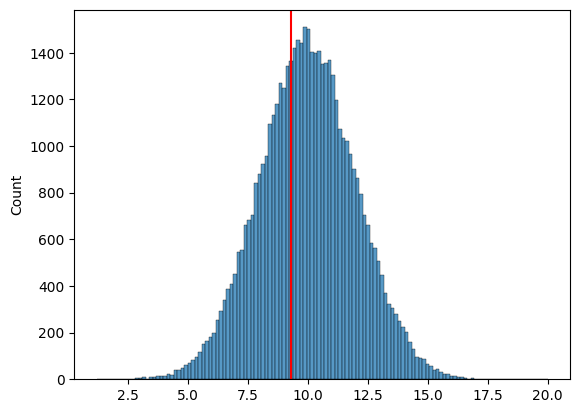
# Make a sample of 10 from the normal distribution
sample = goose_samples[:10]
goose_mean = np.mean(sample)

# in reality, we don't have access to the "true" distribution, which is why it's commented out
sns.histplot(goose_samples)
plt.axvline(x=goose_mean, color='red');
For bootstrap samples, we can use random.Generator.choice() with replacement to draw samples from our dataset.
def mean_estimator(sample):
    """
    An estimator of the expected value E[ ] of the population.

    Args:
        sample (np.array): a sample from the population

    Returns:
        float: the mean of the sample
    """
    return np.mean(sample)
n_samples = 100
true_goose_weight = 10
# in reality, we never know what the distribution actually is
goose_weights = rng.normal(loc=true_goose_weight, scale=2, size=n_samples)
bootstrap_means_list = []
n_bootstraps = 50000

for i in range(n_bootstraps):
    # compute bootstrap sample
    bootstrap_sample = rng.choice(goose_weights, size=100, replace=True)

    # compute our mean
    bootstrap_mean = mean_estimator(bootstrap_sample)
    #print(bootstrap_sample.shape)
    #print(bootstrap_mean)
    # add our bootstrap_mean to a list
    bootstrap_means_list.append(bootstrap_mean)
#len(bootstrap_means_list)
# for i in range(n_bootstraps):
#     # 1. draw a bootstrap sample
#     bootstrap_sample = rng.choice(goose_weights, size=100, replace=True)
#     bootstrap_sample
#     # 2. compute our mean again, with the bootstrap sample
#     bootstrap_mean = mean_estimator(bootstrap_sample)

#     # 3. add our bootstrap_mean to the list
#     bootstrap_means.append(bootstrap_mean)
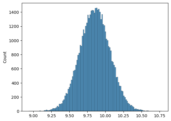
Plotting our bootstrap estimates#
# as our n_bootstraps increase, we're able to see the spread of the estimate
sns.histplot(bootstrap_means_list)
# fix the xaxis to be between 8 and 12
# plt.xlim(8, 12);
<Axes: ylabel='Count'>
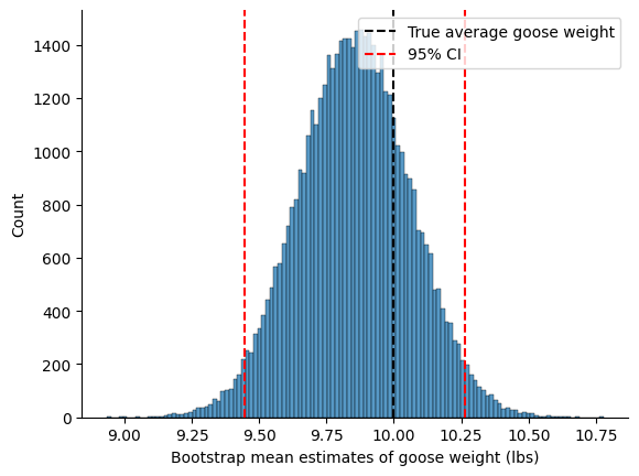
Why we care about uncertainty \(\to\) confidence intervals#
lower_ci = np.percentile(bootstrap_means_list, 2.5)
upper_ci = np.percentile(bootstrap_means_list, 97.5)

print(f"Our estimate of average goose weight: {mean_estimator(goose_weights):.1f} lbs")
print(f"95% Confidence Interval: [{lower_ci:.1f}, {upper_ci:.1f}] lbs")

sns.histplot(bootstrap_means_list)
plt.axvline(true_goose_weight, color='black', linestyle='--', label='True average goose weight')
plt.axvline(lower_ci, color='red', linestyle='--')
plt.axvline(upper_ci, color='red', linestyle='--', label='95% CI')
plt.xlabel('Bootstrap mean estimates of goose weight (lbs)')
plt.gca().spines['top'].set_visible(False)
plt.gca().spines['right'].set_visible(False)
plt.legend()
plt.show()
Our estimate of average goose weight: 9.9 lbs
95% Confidence Interval: [9.4, 10.3] lbs
n_bootstraps = 1000
n_intervals = 1000

count_missed = 0

for j in range(n_intervals):
    # First draw a new sample from the true distribution
    goose_sample = rng.normal(loc=true_goose_weight, scale=2, size=100)

    bootstrap_means = []
    for i in range(n_bootstraps):
        # Draw bootstrap samples from this sample
        bootstrap_sample = rng.choice(goose_sample, size=100, replace=True)
        bootstrap_mean = mean_estimator(bootstrap_sample)
        bootstrap_means.append(bootstrap_mean)

    # Compute CI for this sample
    lower_ci = np.percentile(bootstrap_means, 2.5)
    upper_ci = np.percentile(bootstrap_means, 97.5)

    if true_goose_weight < lower_ci or true_goose_weight > upper_ci:
        count_missed += 1

print(f"Number of intervals that missed the true mean: {count_missed}")
print(f"Proportion of intervals that missed the true mean: {count_missed / n_intervals:.3f}")
Number of intervals that missed the true mean: 55
Proportion of intervals that missed the true mean: 0.055
Why we care about uncertainty \(\to\) comparing estimators#
def first_ten_estimator(sample):
    """
    A (not very good) estimator of the expected value E[ ] of the population.

    Args:
        sample (np.array): a sample from the population

    Returns:
        float: the mean of the first 10 elements of the sample
    """
    return np.mean(sample[:10])
bootstrap_means = []
bootstrap_first_tens = []
n_bootstraps = 5000

# for i in range(n_bootstraps):
#     # 1. draw a bootstrap sample
#     bootstrap_sample = rng.choice(goose_weights, size=100, replace=True)
#     bootstrap_sample

#     # 2. compute our estimates, with the bootstrap sample
#     bootstrap_mean = mean_estimator(bootstrap_sample)
#     bootstrap_first_ten = first_ten_estimator(bootstrap_sample)

#     # 3. add our bootstrap_mean to the list
#     bootstrap_means.append(bootstrap_mean)
#     bootstrap_first_tens.append(bootstrap_first_ten)
# sns.kdeplot(bootstrap_means)#, label="Mean of whole sample")
# sns.kdeplot(bootstrap_first_tens)#, label="Mean of first 10")
# plt.axvline(true_goose_weight, color='black', linestyle='--', label='True average goose weight')
# plt.xlabel('Bootstrap mean estimates of goose weight (lbs)')
# plt.gca().spines['top'].set_visible(False)
# plt.gca().spines['right'].set_visible(False)
# plt.legend()
# plt.show()